| Research article |
|


|
|
|
| Coupling between the Grain for Green Program and a household level-based agricultural eco-economic system in Ansai, Shaanxi Province of China |
LI Yue1, WANG Jijun1,2,*( ), HAN Xiaojia2, GUO Mancai1, CHENG Simin2, QIAO Mei1, ZHAO Xiaocui1 ), HAN Xiaojia2, GUO Mancai1, CHENG Simin2, QIAO Mei1, ZHAO Xiaocui1 |
1 Institute of Soil and Water Conservation, Northwest A&F University, Yangling 712100, China
2 Institute of Soil and Water Conservation, Chinese Academy of Sciences and Ministry of Water Resources, Yangling 712100, China |
|
|
|
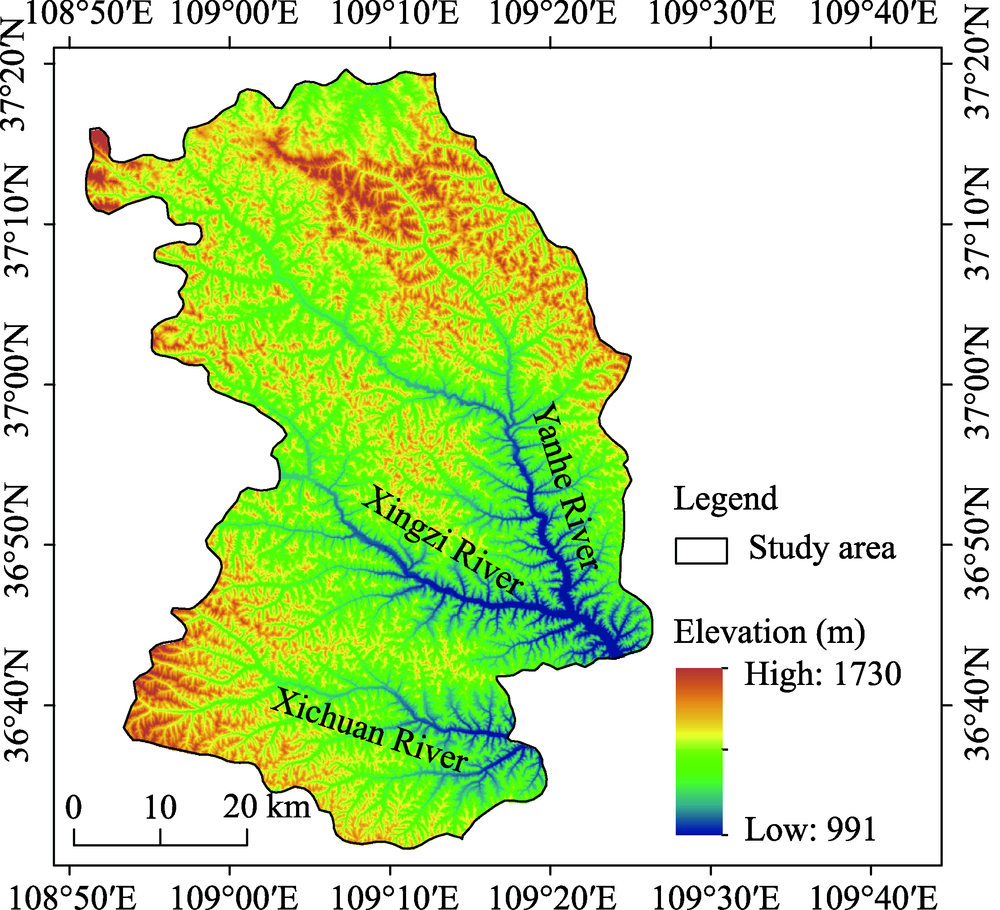
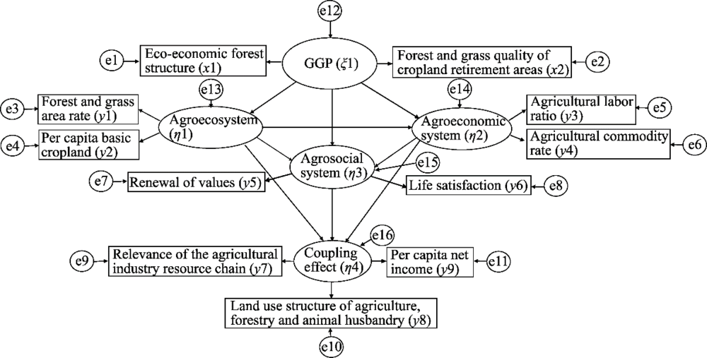
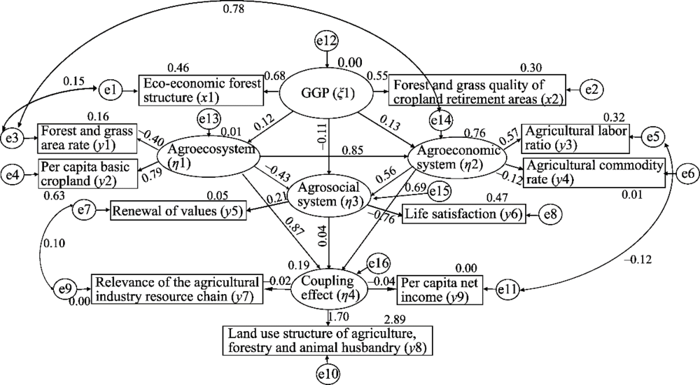
Abstract The implementation of the Grain for Green Program (GGP) has changed the development track of the agricultural eco-economic system in China. In response to the results of a lag study that investigated the coupling between the GGP and the agricultural eco-economic system in a loess hilly region, we used a structural equation model to analyze the survey data from 494 households in Ansai, a district of Yan'an City in Shaanxi Province of China in 2015. The model clarified the direction and intensity of the coupling between the GGP and the agricultural eco-economic system. The coupling benefits were derived through linkages between the program and various chains in the agricultural eco-economic system. The GGP, the agroecosystem of Ansai and their potential coupling effects were in a state of general coordination. The agroecosystem directly affected the coupling effect, with the standardized path coefficient of 0.87, indicating that the agroecosystem in Ansai at this stage provided basic material support for the coupling between the GGP and the agricultural eco-economic system. The direct path coefficient of agroeconomic system impacted on the coupling effect was -0.76, indicating that partial contradictions occurred between the agroeconomic system and the coupling effect. Therefore, although the current agroecosystem in Ansai should be provided sufficient agroecological resources for the benign coupling between the program and the agricultural eco-economic system, agricultural development failed to effectively transform agroecological resources into agricultural economic advantages in this region, which resulted in a relative lag in the development of the agricultural economic system. Thus, the coupling between the GGP and the agricultural eco-economic system was poor. To improve the coupling and the sustainable development of the agricultural eco-economic system in cropland retirement areas, the industrial structure needs to be diversified, the agricultural resources (including agroecological resources, agricultural economic resources and agricultural social resources) need to be rationally allocated, and the chain structure of the agricultural eco-economic system needs to be continuously improved.
|
|
Received: 11 January 2019
Published: 10 March 2020
|
|
Corresponding Authors:
|
| About author: *Corresponding author: WANG Jijun (E-mail: jjwang@ms.iswc.ac.cn) |
|
|
| [1] |
Aderson J C, Gerbring D W. 1988. Structural equation modeling in practice: A review and recommended two-step approach. Pyschological Bulletin, 103(3): 411-423.
doi: 10.1007/s00128-019-02649-3
pmid: 31203410
|
|
|
| [2] |
Asah S T. 2008. Empirical social-ecological system analysis: From theoretical framework to latent variable structural equation model. Environmental Management, 42: 1077-1090.
doi: 10.1007/s00267-008-9172-9
|
|
|
| [3] |
Bennett M T. 2008. China's sloping land conversion program: Institutional innovation or business as usual? Ecological Economics, 65(4): 699-711.
doi: 10.1086/691993
pmid: 29805178
|
|
|
| [4] |
Bertalanffy L V. 1987. General System Theory-Foundation Development, Applications (Reversion edition). New York: George Beazitler, 189-239.
|
|
|
| [5] |
Bollen K A. 1989. Structural Equations with Latent Variables. New York: Wiley, 55-70.
|
|
|
| [6] |
Brahim N, Blavet D, Gallali T, et al. 2011. Application of structural equation modeling for assessing relationships between organic carbon and soil properties in semiarid Mediterranean region. International Journal of Environmental Science & Technology, 8(2): 305-320.
|
|
|
| [7] |
Byrne B M. 1998. Structural Equation Modeling with LISREL, PRELIS, and SIMPLIS; Basic Concepts, Applications, and Programming. Mahwah: Lawrence Erlbaum Associates, 66-74.
|
|
|
| [8] |
Byrne B M. 2001. Structural equation modeling with AMOS, EQS, and LISREL: Comparative approaches to testing for the factorial validity of a measuring instrument. International Journal of Testing, 1(1): 55-86.
doi: 10.1207/S15327574IJT0101_4
|
|
|
| [9] |
Deng L, Liu S, Kim D G, et al. 2017. Past and future carbon sequestration benefits of China's grain for green program. Global Environmental Change, 47: 13-20.
doi: 10.1016/j.gloenvcha.2017.09.006
|
|
|
| [10] |
Duncan T E, Duncan S C, Strycker L A. 2006. An Introduction to Latent Variable Growth Curve Modeling: Concepts, Issues, and Applications. Mahwah: Lawrence Erlbaum Associates, 93-105.
|
|
|
| [11] |
Gough L, Grace J B. 1999. Effects of environmental change on plant species density: Comparing predictions with experiments. Ecology, 80(3): 882-890.
doi: 10.1890/0012-9658(1999)080[0882:EOECOP]2.0.CO;2
|
|
|
| [12] |
Grace J B, Anderson T M, Scheiner O S M. 2010. On the specification of structural equation models for ecological systems. Ecological Monographs, 80(1): 67-87.
doi: 10.1890/09-0464.1
|
|
|
| [13] |
Grosjean P, Kontoleon A. 2009. How sustainable are sustainable development programs? The case of the sloping land conversion program in China. World Development, 37(1): 268-285.
doi: 10.1016/j.worlddev.2008.05.003
|
|
|
| [14] |
Hung N T, Asaeda T, Manatunge J. 2007. Modeling interactions of submersed plant biomass and environmental factors in a stream using structural equation modeling. Hydrobiologia, 583(1): 183-193.
doi: 10.1007/s10750-006-0526-0
|
|
|
| [15] |
Jia X Q, Fu B J, Feng X M, et al. 2014. The trade off and synergy between ecosystem services in the Grain-for-Green areas in Northern Shaanxi, China. Ecological Indicators, 43: 103-113.
doi: 10.1016/j.ecolind.2014.02.028
|
|
|
| [16] |
Kalaitzandonakes N G, Monson M J. 1994. An analysis of potential conservation effort of crp participants in the state of missouri: a latent variable approach. Journal of Agricultural & Applied Economics, 26(1): 200-208.
|
|
|
| [17] |
Li Q R, Wang J J, Guo M C. 2012. Coupling relationship of ecological agricultural system of commodities in Ansai county based on structural equation model. Transactions of the Chinese Society of Agricultural Engineering, 28(16): 240-247. (in Chinese)
|
|
|
| [18] |
Li Q R, Amjath-Babu T S, Zander P, 2016a. Role of capitals and capabilities in ensuring economic resilience of land conservation efforts: A case study of the grain for green project in China's Loess Hills. Ecological Indicators, 71: 636-644.
|
|
|
| [19] |
Li Q R, Liu Z, Zander P, et al. 2016b. Does farmland conversion improve or impair household livelihood in smallholder agriculture system? A case study of Grain for Green project impacts in China's Loess Plateau. World Development Perspectives, 2: 43-54.
doi: 10.1016/j.wdp.2016.10.001
|
|
|
| [20] |
Li Q R, Amjath-Babu T S, Sieber S, et al. 2018. Assessing divergent consequences of payments for ecosystem services (PES) on rural livelihoods: A case-study in China's Loess Hills. Land Degradation & Development, 29(10): 3549-3570.
|
|
|
| [21] |
Li Y, Wang J J, Liu P L, et al. 2018. Study on the synergic relationship between grain for green and agricultural eco-economic social system—A case study in Ansai county. Journal of Natural Resources, 33(7): 1179-1190. (in Chinese)
doi: 10.31497/zrzyxb.20180107
|
|
|
| [22] |
Liu C, Wu B. 2010. Grain for Green Programme in China: Policy making and implementation? Policy Briefing Series, 60: 1-17. The University of Nottingham, China Policy Institute, Nottingham.
doi: 10.1016/j.scitotenv.2016.09.026
pmid: 27623527
|
|
|
| [23] |
Liu J G, Li S X, Ouyang Z Y, et al. 2008. Ecological and socioeconomic effects of China's policies for ecosystem services. Proceedings of the National Academy of Sciences of the United States of America, 105(28): 9477-9482.
|
|
|
| [24] |
Liu J X, Li Z G, Zhang X P, et al. 2013. Responses of vegetation cover to the Grain for Green Program and their driving forces in the He-Long region of the middle reaches of the Yellow River. Journal of Arid Land, 5(4): 511-520.
doi: 10.1007/s40333-013-0177-8
|
|
|
| [25] |
Maruyama G M. 1998. Basics of Structural Equation Modeling. Thousand Oaks: Sage.148-149.
|
|
|
| [26] |
McCune B, Grace L B. 2002. Analysis of Ecological Communities Gleneden Beach. Oregon: MjM Software Design, 1-300.
|
|
|
| [27] |
Persson M, Moberg J, Ostwald M, et al. 2013. The Chinese Grain for Green Programme: Assessing the carbon sequestered via land reform. Journal of Environmental Management, 126: 142-146.
doi: 10.1016/j.jenvman.2013.02.045
|
|
|
| [28] |
Ren J Z, He D H, Wang N, et al. 1995. Models of coupling agro-grassland systems in desert-oasis region. Acta Prataculturae Sinica, 2: 11-19. (in Chinese)
|
|
|
| [29] |
Rong T S.2009. AMOS and Research Methods. Chongqing: Chongqing University Press, 25-33. (in Chinese)
|
|
|
| [30] |
Smith J, Scherr S J. 2003. Capturing the value of forest carbon for local livelihoods. World Development, 31(12): 2143-2160.
doi: 10.1016/j.worlddev.2003.06.011
|
|
|
| [31] |
State Forestry Administration of the People's Republic of China. 2016. China forestry development report 2016, Beijing, China. [2016-12-09]. . (in Chinese)
|
|
|
| [32] |
Steiger J H. 1990. Structural model evaluation and modification: An interval estimation approach. Multivariate Behavioral Research, 25(2): 173-189.
doi: 10.1207/s15327906mbr2502_4
pmid: 26794479
|
|
|
| [33] |
Sutton-Grier A E, Kenney M A, Richardson C J. 2010. Examining the relationship between ecosystem structure and function using structural equation modelling: A case study examining denitrification potential in restored wetland soils. Ecological Modeling, 221(5): 761-768.
doi: 10.1016/j.ecolmodel.2009.11.015
|
|
|
| [34] |
Tomarken A J, Waller N G. 2005. Structural equation modeling: strengths, limitations, and misconceptions. Annual Review of Clinical Psychology, 1(1): 31-65.
doi: 10.1146/annurev.clinpsy.1.102803.144239
pmid: 17716081
|
|
|
| [35] |
Uchida E, Xu J, Rozelle S. 2005. Grain for green: cost-effectiveness and sustainability of China's conservation set-aside programme. Land Economics, 81(2): 247-264.
doi: 10.3368/le.81.2.247
|
|
|
| [36] |
Uchida E, Rozelle S, Xu J. 2009. Conservation payments, liquidity constraints, and off-farm labor: Impact of the Grain-for-Green Program on rural households in China. American Journal of Agricultural Economics, 91(1): 70-86.
doi: 10.1111/ajae.v91.1
|
|
|
| [37] |
Wang J J, Guo M C, Jiang Z D, et al. 2010. The construction and application of an agricultural ecological-economic system coupled process model. Acta Ecological Sinica, 30(9): 2371-2378. (in Chinese)
|
|
|
| [38] |
Wang J J, Wang Z S, Cheng S M, et al. 2017. Eco-economic thinking for developing carbon sink industry in the de-farming regions. Chinese Journal of Applied Ecology, 28(12): 4109-4116. (in Chinese)
doi: 10.13287/j.1001-9332.201712.013
pmid: 29696909
|
|
|
| [39] |
Wang X H, Shen J X, Zhang W. 2014. Emergy evaluation of agricultural sustainability of Northwest China before and after the grain-for-green policy. Energy Policy, 67: 508-516.
doi: 10.1016/j.enpol.2013.12.060
|
|
|
| [40] |
Werner C, Schermelleh-Eagel K. 2009. Structural equation modeling: Advantages, challenges, and problems. Introduction to Structural Equation Modeling with LISREL. Goethe University, Germany.
|
|
|
| [41] |
Wright S. 1934. The method of path coefficients. Annals of Mathematical Statistics, 5(3): 161-215.
doi: 10.1214/aoms/1177732676
|
|
|
| [42] |
Xu Z, Xu J, Deng X, et al. 2006. Grain for Green versus grain: conflict between food security and conservation set-aside in China. World Development, 34(1): 130-148.
doi: 10.1016/j.worlddev.2005.08.002
|
|
|
| [43] |
Yao S, Guo Y, Huo X. 2010. An empirical analysis of the effects of China's land conversion program on farmers' income growth and labor transfer. Environmental Management, 45(3): 502-512.
doi: 10.1007/s00267-009-9376-7
|
|
|
|
Viewed |
|
|
|
Full text
|
|
|
|
|
Abstract
|
|
|
|
|
Cited |
|
|
|
|
| |
Shared |
|
|
|
|
| |
Discussed |
|
|
|
|