| Research article |
|


|
|
|
| Performance and uncertainty analysis of a short-term climate reconstruction based on multi-source data in the Tianshan Mountains region, China |
LI Xuemei1,2,3,*( ), Slobodan P SIMONOVIC4, LI Lanhai5, ZHANG Xueting6,7, QIN Qirui1,3 ), Slobodan P SIMONOVIC4, LI Lanhai5, ZHANG Xueting6,7, QIN Qirui1,3 |
1 Faculty of Geomatics, Lanzhou Jiaotong University, Lanzhou 730070, China
2 National-Local Joint Engineering Research Center of Technologies and Applications for National Geographic State Monitoring, Lanzhou 730070, China
3 Gansu Provincial Engineering Laboratory for National Geographic State Monitoring, Lanzhou 730070, China
4 Facility for Intelligent Decision Support, Department of Civil and Environmental Engineering, Western University, London N6A 3K7, Canada
5 State Key Laboratory of Desert and Oasis Ecology, Xinjiang Institute of Ecology and Geography, Chinese Academy of Sciences, Urumqi 830011, China
6 Qilian Alpine Ecology & Hydrology Research Station, Key Laboratory of Ecohydrology of Inland River Basin, Northwest Institute of Eco-Environment and Resources, Chinese Academy of Sciences, Lanzhou 730000, China
7 University of Chinese Academy of Sciences, Beijing 100049, China |
|
|
|
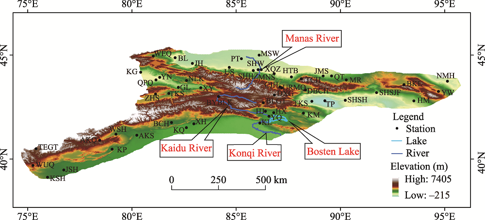
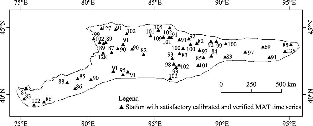
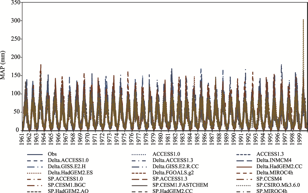
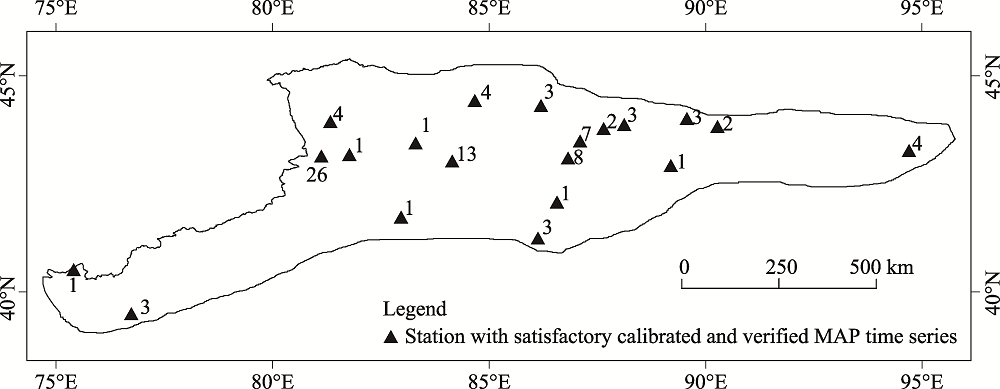
Abstract Short-term climate reconstruction, i.e., the reproduction of short-term (several decades) historical climatic time series based on the relationship between observed data and available longer-term reference data in a certain area, can extend the length of climatic time series and offset the shortage of observations. This can be used to assess regional climate change over a much longer time scale. Based on monthly grid climate data from a Coupled Model Inter-comparison Project phase 5 (CMIP5) dataset for the period of 1850-2000, the Climatic Research Unit (CRU) dataset for the period of 1901-2000 and the observed data from 53 meteorological stations located in the Tianshan Mountains region (TMR) of China during the period of 1961-2011, we calibrated and validated monthly average temperature (MAT) and monthly accumulated precipitation (MAP) in the TMR using the delta, physical scaling (SP) and artificial neural network (ANN) methods. Performance and uncertainty during the calibration (1971-1999) and verification (1961-1970) periods were assessed and compared using traditional performance indices and a revised set pair analysis (RSPA) method. The calibration and verification processes were subjected to various sources of uncertainty due to the influence of different reconstructed variables, different data sources, and/or different methods used. According to traditional performance indices, both the CRU and CMIP5 datasets resulted in satisfactory calibrated and verified MAT time series at 53 meteorological stations and MAP time series at 20 meteorological stations using the delta and SP methods for the period of 1961-1999. However, the results differed from those obtained by the RSPA method. This showed that the CRU dataset produced a low degree of uncertainty (positive connection degree) during the calibration and verification of MAT using the delta and SP methods compared to the CMIP5 dataset. Overall, the calibrated and verified MAP had a high degree of uncertainty (negative connection degree) regardless of the dataset or reconstruction method used. Therefore, the reconstructed time series of MAT for the period of 1850 (or 1901)-1960 based on the CRU and CMIP5 datasets using the delta and SP methods could be used for further study. The results of this study will be useful for short-term (several decades) regional climate reconstruction and longer-term (100 a or more) assessments of regional climate change.
|
|
Received: 16 May 2019
Published: 10 May 2020
|
|
Corresponding Authors:
|
| About author: *Corresponding author: LI Xuemei (E-mail: lixuemei@mail.lzjtu.cn) |
|
|
| [1] |
ASCE Task Committee on Application of Artificial Neural Networks in Hydrology.2000. Artificial neural networks in hydrology I: hydrology application. Journal of Hydrologic Engineering, 5(2): 124-137.
doi: 10.1061/(ASCE)1084-0699(2000)5:2(124)
|
|
|
| [2] |
Beale M H, Hagan M T, Demuth H B.2015. Neural Network Toolbox User's Guide. Natick: The Mathworks Press, 1-906.
|
|
|
| [3] |
Bradley R S, Jones P D.1994. Climate Since A.D. 1500. London: Routledge Press, 511-537.
|
|
|
| [4] |
Cannas B, Fanni A, See L, et al.2006. Data preprocessing for river flow forecasting using neural networks: Wavelet transforms and data partitioning. Physics and Chemistry of the Earth, 31(18): 1164-1171.
|
|
|
| [5] |
Chen H, Xu C Y, Guo S.2012. Comparison and evaluation of multiple GCMs, statistical downscaling and hydrological models in the study of climate change impacts on runoff. Journal of Hydrology, 434-435: 36-45.
|
|
|
| [6] |
Esper J, Cook E R, Schweingruber F H.2002. Low-frequency signals in long tree-ring chronologies for reconstructing past temperature variability. Science, 295(5563): 2250-2253.
doi: 10.1126/science.1066208
|
|
|
| [7] |
Fang K Y, Gou X H, Chen F H.2012. Large-scale precipitation variability over Northwest China inferred from tree rings. Journal of Climate, 25: 1357-1357.
doi: 10.1175/JCLI-D-11-00584.1
|
|
|
| [8] |
Gaur A, Simonovic S P.2017a. Accessing vulnerability of land-cover types to climate change using physical scaling downscaling model. International Journal of Climatology, 37(6): 2901-2912.
doi: 10.1002/joc.2017.37.issue-6
|
|
|
| [9] |
Gaur A, Simonovic S P.2017b. Extension of physical scaling method and its application towards downscaling climate model based near surface air temperature. International Journal of Climatology, 37(8): 3353-3366.
doi: 10.1002/joc.2017.37.issue-8
|
|
|
| [10] |
Ghosh K G.2018. Analysis of rainfall trends and its spatial patterns during the last century over the Gangetic West Bengal, Eastern India. Journal of Geovisualization and Spatial Analysis, 2: 15, doi: 10.1007/s41651-018-0022-x.
doi: 10.1007/s41651-018-0022-x
|
|
|
| [11] |
Gupta H V, Sorooshian S, Yapo P O.1999. Status of automatic calibration for hydrologic models: comparison with multilevel expert calibration. Journal of Hydrologic Engineering, 4(2): 135-143.
doi: 10.1061/(ASCE)1084-0699(1999)4:2(135)
|
|
|
| [12] |
Hao Z H, Li L, Xu Y.2009. Study on Delta-DCSI downscaling method of GCM output. Journal of Sichuan University (Engineering Science Edition), 41(5): 1-7. (in Chinese)
|
|
|
| [13] |
Harris I, Jones P D, Osborn T J, et al.2014. Updated high-resolution grids of monthly climatic observations-the CRU TS3.10 dataset. International Journal of Climatology, 34(3): 623-642.
doi: 10.1002/joc.3711
|
|
|
| [14] |
Hauduc H, Neumann M B, Muschalla D, et al.2015. Efficiency criteria for environmental model quality assessment: A review and its application to wastewater treatment. Environmental Modelling & Software, 68: 196-204.
|
|
|
| [15] |
Hay L E, Wilby I L, Leavesley G H.2000. A comparison of delta change and downscaled GCM scenarios for three mountainous basins in the United States. Journal of the American Water Resource Association, 36(2): 387-397.
doi: 10.1111/jawr.2000.36.issue-2
|
|
|
| [16] |
Hu R J.2004. Physical Geography of the Tianshan Mountains in China. Beijing: China Environmental Science Press, 139-142. (in Chinese)
|
|
|
| [17] |
Huang Y, Yan Q, Zhang C.2018. Spatial-temporal distribution characteristics of PM 2.5, in China in 2016. Journal of Geovisualization and Spatial Analysis, 2(2): 1-18.
doi: 10.1007/s41651-017-0008-0
|
|
|
| [18] |
Klippel L, Krusic P J, Brandes R, et al.2018. A 1286-year hydro-climate reconstruction for the Balkan Peninsula. Boreas, 47(4): 1218-1229.
doi: 10.1111/bor.2018.47.issue-4
|
|
|
| [19] |
Levenberg K.1944. A method for the solution of certain non-linear problems in least squares. The Quarterly of Applied Mathematics, 2: 164-168.
doi: 10.1090/qam/1944-02-02
|
|
|
| [20] |
Li X M, Li L H, Wang X X, et al.2013. Reconstruction of hydrometeorological time series and its uncertainties for the Kaidu River Basin using multiple data sources. Theoretical and applied climatology, 113: 45-62.
doi: 10.1007/s00704-012-0771-2
|
|
|
| [21] |
Li X M, Gao P, Li Q, Tang H.2016. Muti-paths impact from climate change on snow cover in Tianshan Mountainous area of China. Advance in Climate Change Research, 12(4): 303-312. (in Chinese)
|
|
|
| [22] |
Liu X K, Rao Z G, Zhang X J, et al.2015. Variations in the oxygen isotopic composition of precipitation in the Tianshan Mountains region and their significance for the Westerly circulation. Journal of Geographical Sciences, 25(7): 801-816.
doi: 10.1007/s11442-015-1203-x
|
|
|
| [23] |
Marquardt D.1963. An algorithm for least-squares estimation of nonlinear parameters. SIAM Journal on Applied Mathematics, 11(2): 431-441.
|
|
|
| [24] |
Misra V, DiNapoli S M, Bastola S.2012. Dynamic downscaling of the twentieth-century reanalysis over the southeastern United States. Regional Environment Change, 13: 15-23.
doi: 10.1007/s10113-012-0372-8
|
|
|
| [25] |
Moriasi D N, Arnold J G, van Liew M W, et al.2007. Model evaluation guidelines for systematic quantification of accuracy in watershed simulations. Transactions of the American Society of Agricultural and Biological Engineers, 50(3): 885-900.
|
|
|
| [26] |
Nash J E, Sutcliffe J V.1970. River fiow forecasting through conceptual models Part 1: A discussion of principles. Journal of Hydrology, 10(3): 282-290.
doi: 10.1016/0022-1694(70)90255-6
|
|
|
| [27] |
Nourani V, Komasi M, Mano A.2009. A multivariate ANN-wavelet approach for rainfall-runoff modeling. Water Resources Management, 23: 2877-2894.
doi: 10.1007/s11269-009-9414-5
|
|
|
| [28] |
Pi H, Sharratt B, Feng G, et al.2017. Evaluation of two empirical wind erosion models in arid and semi-arid regions of China and the USA. Environmental Modelling & Software, 91: 28-46.
|
|
|
| [29] |
Schimek M G, Turlach B A.2000. Additive and generalized additive models. In: Schimek M G. Smoothing and Regression: Approaches, Computation, and Application. New York: Wiley Press, 277-327.
|
|
|
| [30] |
Shen J, Zhang E L, Xia W L.2001. Records from lake sediments of the Qinghai Lake to mirror climatic and environmental changes of the past about 1000 years. Quaternary Sciences, 21(6): 508-514.
|
|
|
| [31] |
Shen S S P, Clarke G, Shen B W, et al.2019. Spatiotemporal variations of the twentieth century Tibetan Plateau precipitation based on the monthly 2.5° reconstructed data. Theoretical and Applied Climatology, 135: 71-83.
doi: 10.1007/s00704-017-2357-5
|
|
|
| [32] |
Shi Y, Shen Y, Kang E, et al.2007. Recent and future climate change in northwest China. Climate Change, 80: 379-393.
doi: 10.1007/s10584-006-9121-7
|
|
|
| [33] |
Srinivasulu S, Jain A.2006. A comparative analysis of training methods for artificial neural network rainfall-runoff models. Applied Soft Computing, 6: 295-306.
doi: 10.1016/j.asoc.2005.02.002
|
|
|
| [34] |
Su M R, Yang Z F, Chen B, et al.2009. Urban ecosystem health assessment based on energy and set pair analysis—a comparative study of typical Chinese cities. Ecological Modelling, 220(18): 2341-2348.
doi: 10.1016/j.ecolmodel.2009.06.010
|
|
|
| [35] |
Taylor K E, Stouffer R J, Meehl G A.2012. A summary of the CMIP5 experiment design. Bulletin of the American Meteorological Society, 93(4): 485-498.
doi: 10.1175/BAMS-D-11-00094.1
|
|
|
| [36] |
University of East Anglia Climatic Research Unit, Harris I C, Jones P D.2020. CRU TS4.03: Climatic Research Unit (CRU) Time-Series (TS) version 4.03 of high-resolution gridded data of month-by-month variation in climate (Jan. 1901-Dec. 2018). [2020-01-22]. Centre for Environmental Data Analysis, doi: 10.5285/10d3e3640f004c578403419aac167d82.
|
|
|
| [37] |
Wang G Q, Zhao K Q, Zhen X J.2004. Application of set pair analysis to fuzzy predictors of multiple regression weather forecast models. Bulletin of Science and Technology, 20(2): 151-155. (in Chinese)
|
|
|
| [38] |
Wang H Q, Chen F, Ermenbaev B, et al.2017. Comparison of drought-sensitive tree-ring records from the Tien Shan of Kyrgyzstan and Xinjiang (China) during the last six centuries. Advances in Climate Change Research, 8(1): 18-25.
doi: 10.1016/j.accre.2017.03.004
|
|
|
| [39] |
Wang M W, Wei D F, Li J, et al.2014. A novel clustering model based on set pair analysis for the energy consumption forecast in China. Mathematical Problems in Engineering, 2014(1): 1-8, doi: 10.1155/2014/191242.
|
|
|
| [40] |
Wang W S, Xiang H L, Li Y Q, et al.2008. A new approach to annual runoff classification based on set pair analysis. Journal of Sichuan University (Engineering Science Edition), 40(5): 1-6. (in Chinese)
|
|
|
| [41] |
Wang W S, Jin J L, Ding J, et al.2009. A new approach to water resources system assessment-set pair analysis method. Science in China Series E: Technological Sciences, 52(10): 3017-3023.
doi: 10.1007/s11431-009-0099-z
|
|
|
| [42] |
Wang W S, Li Y Q.2012. Hazard degree assessment of landslide using set pair analysis method. Natural Hazards, 60(2): 367-379.
doi: 10.1007/s11069-011-0017-0
|
|
|
| [43] |
Wei W S, Yuan Y J, Yu S L, et al.2008. Climate change in recent 235 years and trend prediction in Tianshan Mountainous area. Journal of Desert Research, 28(5): 803-808. (in Chinese)
|
|
|
| [44] |
Wood S N.2000. Modelling and smoothing parameter estimation with multiple quadratic penalties. Journal of the Royal Statistical Society: Series B (Statistical Methodology), 62(2): 413-428.
doi: 10.1111/rssb.2000.62.issue-2
|
|
|
| [45] |
Wu Z T, Zhang H J, Krause C M, et al.2010. Climate change and human activities: a case study in Xinjiang, China. Climatic Change, 99: 457-472.
doi: 10.1007/s10584-009-9760-6
|
|
|
| [46] |
Yan F, Xu K, Li D, et al.2017. A novel hazard assessment method for biomass gasification stations based on extended set pair analysis. PLoS ONE, 12(9): e0185006.
doi: 10.1371/journal.pone.0185006
|
|
|
| [47] |
Yang B, Braeuning A, Johnson K R, et al.2002. General characteristics of temperature variation in China during the last two millennia. Geophysical Research Letters, 29(9): 1029-1040.
doi: 10.1029/2001GL013866
|
|
|
| [48] |
Yang J J, Zhou J Z, Liu L, et al. Similarity Measures between Connection Numbers of Set Pair Analysis. In: Sun F, Zhang J, Tan Y, et al. Advances in Neural Networks - ISNN 2008. ISNN 2008. Lecture Notes in Computer Science, Vol. 5263. Berlin, Heidelberg: Springer, 63-68.
|
|
|
| [49] |
Yao T, Masson-Delmotte V, Gao J, et al.2013. A review of climatic controls on delta 18O in precipitation over the Tibetan Plateau: observations and simulations. Review of Geophysics, 51(4): 525-548.
doi: 10.1002/rog.v51.4
|
|
|
| [50] |
Ye Y C, Wu Y L.2000. The set pair analysis for the comprehensive evaluation of mine operation state. Metal Mine, 6: 23-33. (in Chinese)
|
|
|
| [51] |
Zhang F Y, Ahmad S, Zhang H Q, et al.2016a. Simulating low and high streamflow driven by snowmelt in an insufficiently gauged alpine basin. Stochastic Environmental Research and Risk Assessment, 30: 59-75.
doi: 10.1007/s00477-015-1028-2
|
|
|
| [52] |
Zhang F Y, Bai L, Li L H, et al.2016b. Sensitivity of runoff to climatic variability in the northern and southern slopes of the Middle Tianshan Mountains, China. Journal of Arid Land, 8(5): 681-693.
doi: 10.1007/s40333-016-0015-x
|
|
|
| [53] |
Zhang X T, Li X M, Li L H, et al.2019. Environmental factors influencing snowfall and snowfall prediction in the Tianshan Mountains, Northwest China. Journal of Arid Land, 11(1): 15-28.
doi: 10.1007/s40333-018-0110-2
|
|
|
| [54] |
Zhao F F, Xu Z X.2007. Comparative analysis on downscaled climate scenarios for headwater catchment of Yellow River using SDS and Delta methods. Acta Meteorologica Sinica, 65(4): 653-662. (in Chinese)
doi: 10.11676/qxxb2007.060
|
|
|
| [55] |
Zhao K Q.1989. Set pair and set pair analysis-a new concept and systematic analysis method. In: Proceedings of the National Conference on System Theory and Regional Planning. Baotou, China, 87-91. (in Chinese)
|
|
|
| [56] |
Zhao K Q, Xuan A L.1996. Set pair theory-a new theory method of non-define and its applications. Systems Engineering, 14(1): 18-23. (in Chinese)
|
|
|
| [57] |
Zhou J X, Li X M, Chen L, et al.2007. Updating methods for dynamic assessment of ecological footprint-a case study of Wuhan City. Resources Science, 29(3): 111-116. (in Chinese)
|
|
|
|
Viewed |
|
|
|
Full text
|
|
|
|
|
Abstract
|
|
|
|
|
Cited |
|
|
|
|
| |
Shared |
|
|
|
|
| |
Discussed |
|
|
|
|